密度の算出方法#

液体の密度はNPT計算を行うことで算出出来ます。

まずは水の密度を求めてみます。

水分子の用意#

はじめに、計算する水分子のパラメータを設定します。

今回はSPC/E力場パラメータを使って密度を計算してみましょう。

水の力場とそれを使ったlammpsスクリプトがLAMMPSのマニュアルに記載があるので、この内容を参考にして書いていきます。

units real

・1行目はスクリプト内で使う単位系を設定しています。

今回使っているrealという単位系は、例えば質量の単位が \(g/mol\) なので、7行目のmassコマンドで設定している数値は \(15.9996 g/mol\) を意味しています。 units (lammps ドキュメント)

・次に2行目ですが、これは原子一個一個にどんな値を設定できるか(atom_style)を決めています。

atom_style full

このスクリプトでのatom_styleはfullなので、次のような数値を設定することが可能です。設定しなくても構いません。

atom-ID ：各原子の名前
type ：識別ID
position ：座標 x,y,z
velosity ：速度 vx,vy,vz
force ：働く力 fx,fy,fz
image-frags：可視化のための数値データ
mask ：所属するグループ名
bond ： 2原子間の力場パラメータデータ
angle ： 3原子間の力場パラメータデータ
dihedral ： 4原子間の力場パラメータデータ
improper ：以上以外の構造における力場パラメータデータ
charge ：各原子の電荷

atom_style (lammps ドキュメント)

このページでは特別な理由がない限り*unit real*を用いることにします。

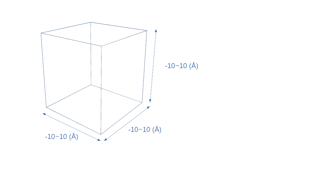
・次に3行目、この行ではregionコマンドを使って水分子を配置するボックスの大きさを設定しています。この設定ではちょうど以下の画像で描いた領域が計算セルボックスになります。

region box block -10 10 -10 10 -10 10

コードの意味は、左から

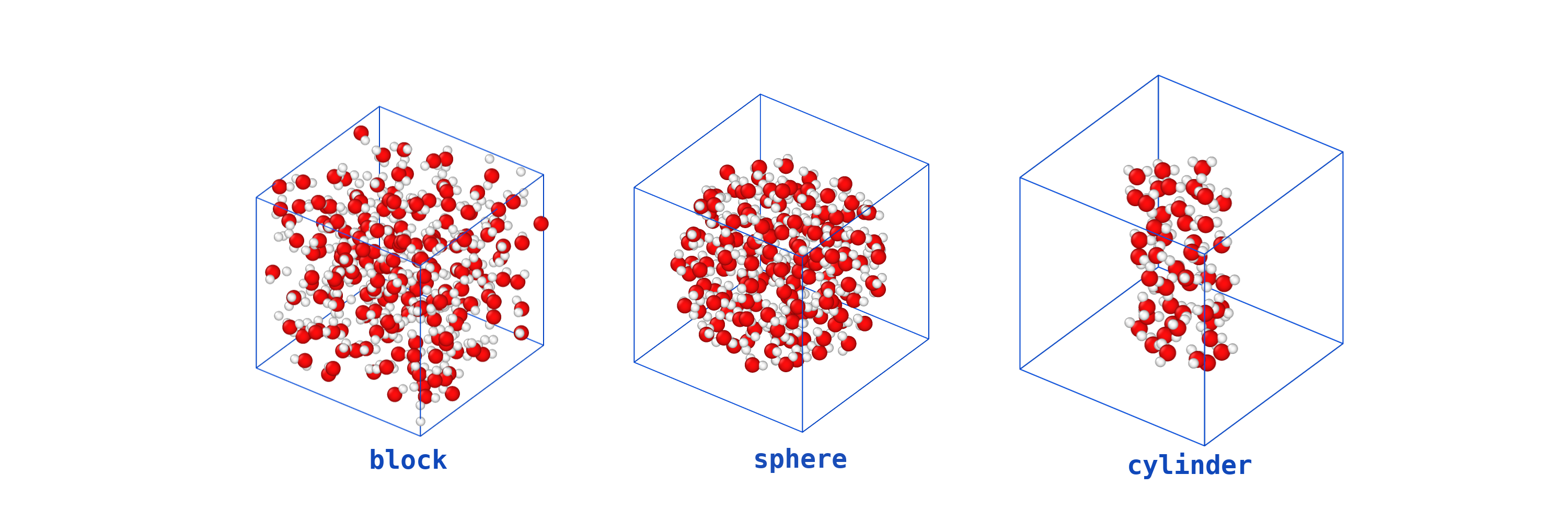
region 領域名領域の型型に合わせた設定値

となります。 region (lammps ドキュメント) を見ると、領域の型はcylinderやsphereを選べるようなので、水分子の集団を球で配置したい場合はsphereを使うということになります。 block,sphere,cylinderそれぞれの設定にした場合、次のような初期配置を作ることが出来ます。

・次の4行目は、”計算セル”どれくらいの原子種(atom_type)、結合種(bond_type)、・・・を入れることにするかを設定しています。このcreate_boxコマンドはregionコマンドで作成した領域を使いますが、今回は3行目で作成したboxという領域を使っています。

create_box 2 box  bond/types 1 angle/types 1 &
            extra/bond/per/atom 2 extra/angle/per/atom 1 extra/special/per/atom 2

コマンドの意味は

create_box 原子種の数領域名 bond/types 結合数 angle/types 角度の数 (必要ならば dihedral/types 二面角の数 improper/types その他の結合の数)

を表します。（extra/...はまだ理解してません。。。）

・次に力場の形式とパラメータを設定しています。

mass 1 15.9994 #質量の設定
mass 2 1.008

pair_style lj/cut/coul/long 10.0  #原子同士の結合力の設定
bond_style zero  #2原子間の結合力
angle_style zero  #3原子間の結合力
kspace_style pppm 1e-6

# 力場パラメータ
pair_coeff 1 1 0.1553 3.166
pair_coeff 1 2 0.0    1.0
pair_coeff 2 2 0.0    1.0
bond_coeff 1 1.0
angle_coeff 1 109.47

これだけでは水分子の原子の位置などがまだ定義されていません。原子の位置的な情報は以下のテキストをspc.molとして保存しておきます。

# Water molecule. SPC/E geometry

atoms
bonds
angles

Coords

  0.00000  -0.06461   0.00000
  0.81649   0.51275   0.00000
 -0.81649   0.51275   0.00000

Types

      1   # O
      2   # H
      2   # H

Charges

     -0.8476
      0.4238
      0.4238

Bonds

 1      1      2
 1      1      3

Angles

 1      2      1      3

Shake Flags

1
1
1

Shake Atoms

1 2 3
1 2 3
1 2 3

Shake Bond Types

1 1 1
1 1 1
1 1 1

Special Bond Counts

2 0 0
1 1 0
1 1 0

Special Bonds

2 3
1 3

水分子の空間配置#

ここまでで水分子については設定出来たので、続いて水分子を領域に配置しましょう。スクリプトファイルにコマンドを書き加えていきます。

molecule water spce.mol
create_atoms 0 random 300 34564 NULL mol water 25367 overlap 1.33

・moleculeコマンドで水分子の位置情報をspce.molファイルから読み取ってwaterという名前をつけています。

・create_atomsコマンドで実際にある領域に分子を配置します。この一行で挿入する分子の数、挿入する領域、挿入する分子、重ならない距離の設定を行っています。コマンド内で何を設定しているかはドキュメントを見るのが最もわかりわすいと思います。

create_atoms(lammpsドキュメント)

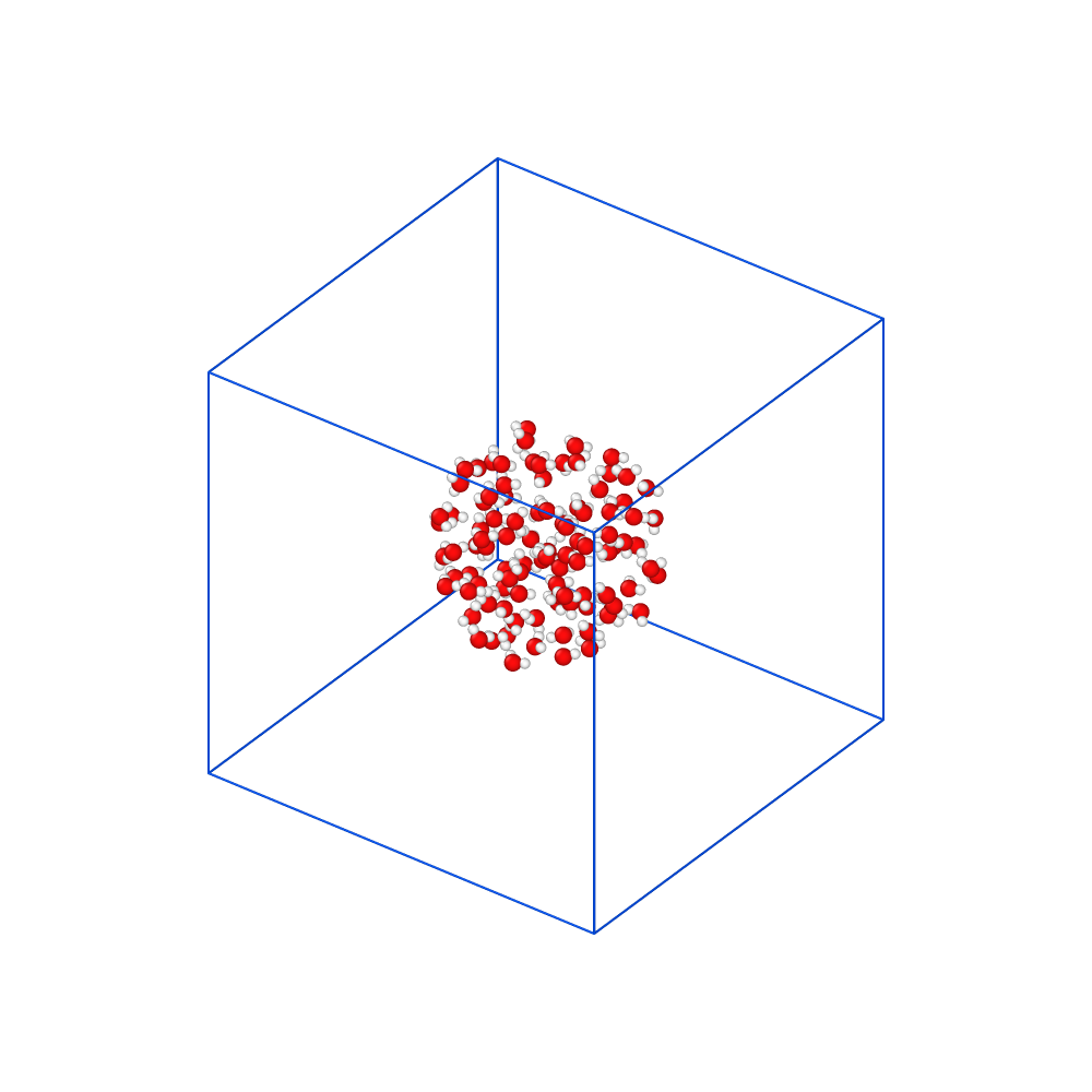
今回のコードでは領域を設定する箇所がNULLとなっており、先程設定したcreate_boxコマンドで作った計算領域全体に水分子が配置されます。しかし、ここで新たに用意した領域を使うと空間の一部に配置することも可能です。

units real
atom_style full
region box block -20 20 -20 20 -20 20
region sphere sphere 0 0 0 10 side in
#region cylinder cylinder z 0 0 4 -10 10 side in

create_box 2 box bond/types 1 angle/types 1 &
                extra/bond/per/atom 2 extra/angle/per/atom 1 extra/special/per/atom 2

~~~
~~~

molecule water spce.mol
create_atoms 0 random 100 34564 sphere mol water 25367 overlap 1.5

ここまでで水分子の空間配置が完了しました。一度スクリプト全体を見てみます。

units real
atom_style full
region box block -5 5 -5 5 -5 5
create_box 2 box  bond/types 1 angle/types 1 &
                extra/bond/per/atom 2 extra/angle/per/atom 1 extra/special/per/atom 2

mass 1 15.9994 #質量の設定
mass 2 1.008

pair_style lj/cut/coul/long 10.0  #原子同士の結合力の設定
bond_style zero  #2原子間の結合力
angle_style zero  #3原子間の結合力
kspace_style pppm 1e-6

# 力場パラメータ
pair_coeff 1 1 0.1553 3.166
pair_coeff 1 2 0.0    1.0
pair_coeff 2 2 0.0    1.0
bond_coeff 1 1.0
angle_coeff 1 109.47

molecule water spce.mol
create_atoms 0 random 33 34564 NULL mol water 25367 overlap 1.33

MD計算の設定#

・続いて計算タイムステップを設定します。

timestep 1.0

今単位系はrealなので時間の単位はフェムト秒です。したがって時間ステップは1フェムト秒と設定していることを意味しています。

・次に水分子のOH振動とHOH偏角の運動を固定します。今回使用したSPCモデルはこの固定をした上でチューニングされているそうです。

その証拠に、先に設定した結合と角度のパラメータには距離と角度の値しかなく、振動中心のようなその他のパラメータはありません。

shakeアルゴリズム（ shake(lammpsドキュメント) ）を用いることで結合と角度を固定出来ます。

fix water_fix all shake 0.0001 10 1000 b 1 a 1

コマンド内の b 1 a 1 は結合の1番目、角度1番目を固定するとこを示しています。

・NPT計算の設定を行います。ここでは全ての原子の平均温度が300Kに、圧力を1stmに温度調整・圧力調整する設定になっています。

fix integrate all npt temp 300.0 300.0 100.0 iso 1.0 1.0 1000.0

・分子の運動を記録するために、トラジェクトリを記録する設定を行います。全てno原子のトラジェクトリを100ステップごとにdump.lammpstrjというファイルに出力する設定になっています。

dump myDump all atom 100 dump.lammpstrj

・log.lammpsファイルにおける出力する数値を設定します。右から時間ステップ数、温度、圧力、全エネルギー、密度、ポテンシャルエネルギー、運動エネルギーです。つまりここで密度の時系列データが出力できることになります。

thermo 1000 とは100ステップごとに上記の値を出力することを示しています。

thermo_style custom step temp press etotal density pe ke
thermo 100

・計算ステップ数を設定します。

run 20000

・最後に計算後の系を出力します。

write_data spce.data

ここまでで密度を計算するためのスクリプトが出来ました。

完成したものを以下に表示します。

units real
atom_style full
region box block -10 10 -10 10 -10 10
create_box 2 box  bond/types 1 angle/types 1 &
                extra/bond/per/atom 2 extra/angle/per/atom 1 extra/special/per/atom 2

mass 1 15.9994 #質量の設定
mass 2 1.008

pair_style lj/cut/coul/long 10.0  #原子同士の結合力の設定
bond_style zero  #2原子間の結合力
angle_style zero  #3原子間の結合力
kspace_style pppm 1e-6

# 力場パラメータ
pair_coeff 1 1 0.1553 3.166
pair_coeff 1 2 0.0    1.0
pair_coeff 2 2 0.0    1.0
bond_coeff 1 1.0
angle_coeff 1 109.47

molecule water spce.mol
create_atoms 0 random 300 34564 NULL mol water 25367 overlap 1.33

timestep 1.0
minimize 0.0 0.0 1000 10000
fix integrate all npt temp 300.0 300.0 100.0 iso 1.0 1.0 1000.0

dump myDump all atom 100 dump.lammpstrj

thermo_style custom step temp press etotal density pe ke
thermo 100
run 20000

write_data spce.data

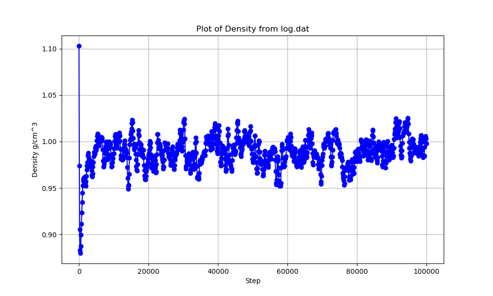
このコードを実行すると密度はこのような変動をします。

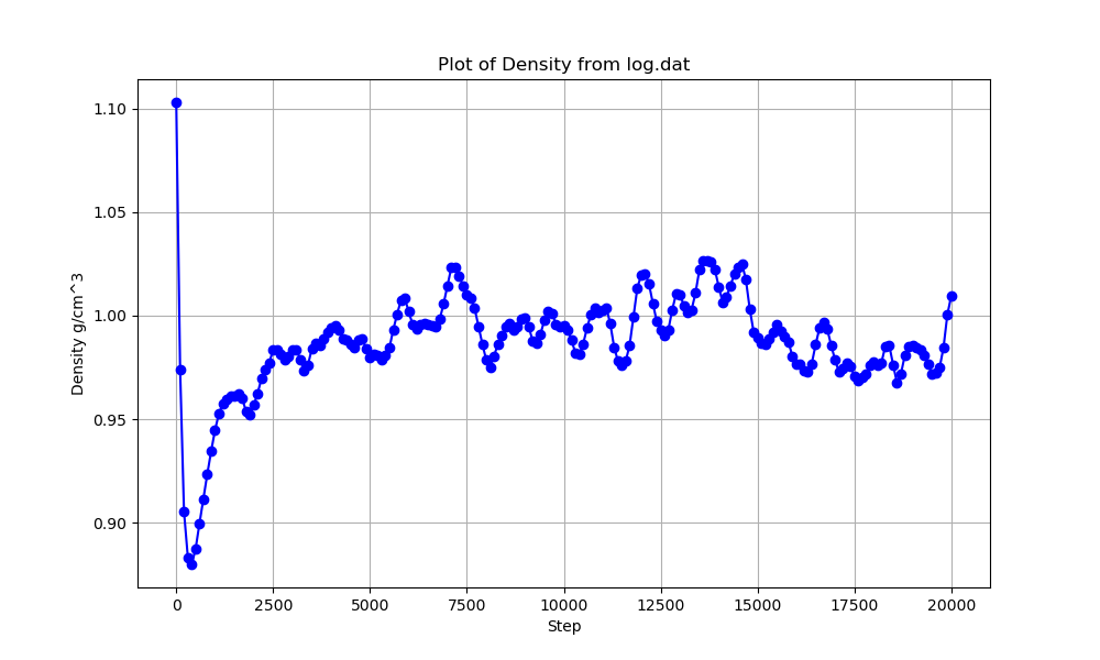
計算時間を100000ステップにするとこんな感じ。

補足#

上のプロットに使用したpythonコード

import matplotlib.pyplot as plt
import numpy as np

file_path = 'log.lammps'

# Read the file and display the first few lines to understand its structure
with open(file_path, 'r') as file:
    lines = file.readlines()

# Define the start and end markers
start_marker = "Step"
end_marker = "Loop time of"

# Initialize flags and container for the relevant lines
capture = False
relevant_lines = []

# Iterate through each line to capture the relevant part
for line in lines:
    if start_marker in line:
        capture = True
    if end_marker in line:
        capture = False
        break  # Stop capturing after finding the end marker and do not include this line
    if capture:
        relevant_lines.append(line)
import matplotlib.pyplot as plt
import numpy as np
# Path for the new file to save the extracted content
output_file_path = 'log.dat'

# Save the extracted lines to the new file
with open(output_file_path, 'w') as output_file:
    output_file.writelines(relevant_lines)

# Provide the path to the saved file


data_path = output_file_path
data_with_header_updated = np.genfromtxt(data_path, names=True, usecols=(0, 4))

# Extracting the updated column names for labels
updated_column_names = data_with_header_updated.dtype.names

# Re-plotting with the updated columns
plt.figure(figsize=(10, 6))
plt.plot(data_with_header_updated[updated_column_names[0]], data_with_header_updated[updated_column_names[1]], marker='o', linestyle='-', color='blue')
plt.title(f'Plot of {updated_column_names[1]} from log.dat')
plt.xlabel(updated_column_names[0])
plt.ylabel(updated_column_names[1]+" g/cm^3")
plt.grid(True)
plt.show()